Processing Vaisala Radiosonde data with Python, and creating GRUAN-like NetCDF files
One of my last projects involved parsing a few GB’s of data that was in a certain binary format, and convert it into NetCDF files. In this post I will describe what was done, what I learned about radiosonde, GRUAN and other geek stuff. Ready?
Vaisala Radiosonde data
When I was told the data was in some binary format, I thought it would be similar to parsing a flat file. That this would contain a fixed length entry, with the same kind of item repeated multiple times.
Well, not exactly.
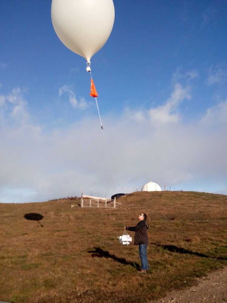
The files had been generated by an instrument made by Vaisala, a Finnish company. This instrument is called a radiosonde. It is an instrument about the size of an old mobile phone, that is launched with a balloon into the atmosphere.
I was lucky to be given the chance to release one of these balloons carrying a newer version of this equipment.

The balloon can carry equipments for measuring different things, like air pressure, altitude, temperature, latitude, longitude, relative humidity, among others. Equipments like the radiosonde send the data back to a ground-level station via radio, normally in a short and constant interval.
The data that I had to parse was Vaisala radiosonde data. But in an older format. The documentation for the format can be found online at http://badc.nerc.ac.uk/data/ukmo-rad-hires/pc-coradata.html.
There are four different sections. And one field in the identification section defines the number of entries found in another field (high resolution). Each section has multiple fields, with different data types.
Not so easy to parse…
Parsing binary data with Python and construct
Construct is a declarative parser for binary data. You can build a parser by simply saying what you expect to be in each field. For example.
pccora_header = Struct("pccora_header",
    ExprAdapter(String("copyright", 20),
        encoder = lambda obj, ctx: obj.encode(),
        decoder = lambda obj, ctx: obj.decode('utf-8', 'ignore')
    ),
    SLInt16("identification_length"),
    SLInt16("syspar_length"),
    SLInt16("data_records"),
    SLInt16("standard_levels"),
    SLInt16("data_type"),
    SLInt16("data_length"),
    Enum(Byte("file_ready"),
        READY = 1,
        NOT_READY = 0,
        _default_ = "UNKNOWN",
    ),
    Bytes("reserved", 17)
)
This sample code parses the Header section of the Vaisala binary file. You define each field, with a short name, a data type and a length. You can also have expressions to encode or decode. And you can control how fields relate to each other, and how they repeat in the data format.
A complete parser for the binary format was written with Construct, and is available
via pip as well, as a package called pccora. You can
install it via pip install pccora, and use it to parse any data in this old binary
format.
There are utility scripts in the pccora GitHub project. One of the scripts, convert2netcdf.py, converts the Vaisala binary data into a NetCDF that is close to what GRUAN produces.
What is GRUAN, and why should I care?

This part of the post is more climate and research-oriented. So if you are more geek-savvy, feel free to jump to the next section.
GRUAN stands for Global Climate Observing System (GCOS) Reference Upper-Air Network (GRUAN).
It is a group of professionals and researchers that work together to create a reference network for climate records. They provide data in a standardised way, and with a uniform quality control process.
This makes it much easier for researchers to use and share data in their work, since they can write tools and scripts once for GRUAN data. Also, there is a quality control process, and every data is annotated with metadata.
Producing NetCDF files with Python
NetCDF, the Network Common Data Form, is a data format that supports arrays with dimensions. Version 4 of NetCDF supports HDF5 too, which is a hierarchical data format.
In NetCDF, you create variables, which contains an array of values - or missing values. These variables relate to one or more dimensions, like time, or altitude.
As for radiosonde data, we have NetCDF files created by GRUAN certified sites. Like this example from NOAA. Following the Download link you should be directed to the FTP site. There you can grab any example GRUAN NetCDF (.nc) file and inspect with ncdump, Panoply, ncBrowse or your favourite editor.
For the file for example, the time and pressure variables are described below.
dimensions:
  time = UNLIMITED ; // (5735 currently)
variables:
  float time(time) ;
    time:standard_name = "time" ;
    time:units = "seconds since 2016-01-03T23:30:16" ;
    time:long_name = "Time" ;
    time:g_format_type = "FLT" ;
    time:g_format_format = "F8.1" ;
    time:g_format_width = "8" ;
    time:g_format_nan = "NaN" ;
    time:g_source_desc = "FRAWPTU" ;
    time:g_column_type = "original data" ;
    time:g_resolution = "1.0 s (time)" ;
    time:axis = "T" ;
    time:calendar = "gregorian" ;
  float press(time) ;
    press:standard_name = "air_pressure" ;
    press:units = "hPa" ;
    press:long_name = "Pressure" ;
    press:g_format_type = "FLT" ;
    press:g_format_format = "F8.3" ;
    press:g_format_width = "8" ;
    press:g_format_nan = "NaN" ;
    press:g_processing_flag = "raw, smoothed, internal QC passed, additional QC passed" ;
    press:g_source_desc = "FRAWPTU" ;
    press:g_column_type = "original data" ;
    press:g_resolution = "15.0 s (time)" ;
    press:comment = "Barometric air pressure using silicon sensor up to 13.1 km, derived from GPS-altitude above" ;
    press:related_columns = "u_press " ;
    press:coordinates = "lon lat alt" ;
You can see the unit used for time (in seconds) and that the time variable is related to the launch time. And pressure is using hPa. Both variables are mapped against the time dimension - you can see that by looking at the parenthesis that follow the variable name.
The following snippet contains an example of the metadata that is added to data uploaded to GRUAN.
// global attributes:
    :Conventions = "CF-1.4" ;
    :title = "RS92 GRUAN Data Product (Version 2)" ;
    :institution = "JMA - Japan Meteorological Agency" ;
    :source = "RS92-SGP" ;
    :history = "2016-01-04 13:10:41.000Z RS92-GDP: RS92 GRUAN Data Product with gruan_DP_calcRsDataProduct.pro (GRUAN IDL Library, 2012-08)" ;
    :references = "Currently no references" ;
    :comment = "RS92 GRUAN Data Product" ;
    :g.Product.ID = "180821" ;
    :g.Product.Code = "RS92-GDP" ;
    :g.Product.Name = "RS92 GRUAN Data Product" ;
    :g.Product.Version = "2" ;
    :g.Product.Level = "2" ;
    :g.Product.LevelDescription = "Data read from original data file" ;
    :g.Product.History = "2016-01-04 13:10:41.000Z RS92-GDP: RS92 GRUAN Data Product with gruan_DP_calcRsDataProduct.pro (GRUAN IDL Library, 2012-08)" ;
    :g.Product.References = "Currently no references" ;
    :g.Product.Producer = "GRUAN Lead Centre (Lindenberg, DWD, Germany)" ;
For my work, the pccora Python library handled the binary data. I created a local variable, hires_data that holds the high resolution data from the radiosonde. Then created a new dataset, which is the NetCDF file.
It might be easier to explain the rest after looking at some code.
hires_data = data['hires_data']

dataset = Dataset(file, "w", format="NETCDF4_CLASSIC")

# Dimensions
dataset.createDimension("time")

dataset.setncattr('g.General.SiteWmoId', ident['wmo_block_number'] + ident['wmo_station_number'])
dataset.setncattr('g.MeasuringSystem.Longitude', str('N/A' if None == ident['station_longitude'] else ident['station_longitude']) + ' degree east')
dataset.setncattr('g.MeasuringSystem.Latitude', str(ident['station_latitude']) + ' degree north')
In this example, a time dimension is added to our dataset, as well as some global attributes (metadata).
In another part of the code, we have to populate arrays with the values for the data logged during the time, and then create variables to persist this data in the NetCDF file.
# elapsed_time
elapsed_time_variable = dataset.createVariable('elapsed_time', 'f4', ("time", ), zlib=True, fill_value=-32768)
elapsed_time_variable.standard_name = 'elapsed_time'
elapsed_time_variable.units = 's'
elapsed_time_variable.long_name = 'Elapsed time since sonde release'
elapsed_time_variable.g_format_type = 'FLT'
elapsed_time_variable[:] = elapsed_time
In this example, elapsed_time is a simple Python array, with float values.
The complete code is available on GitHub.
And once we have parsed the binary data, created the right structures in Python, persisted the new data as NetCDF, we can use it with other tools and programming languages.
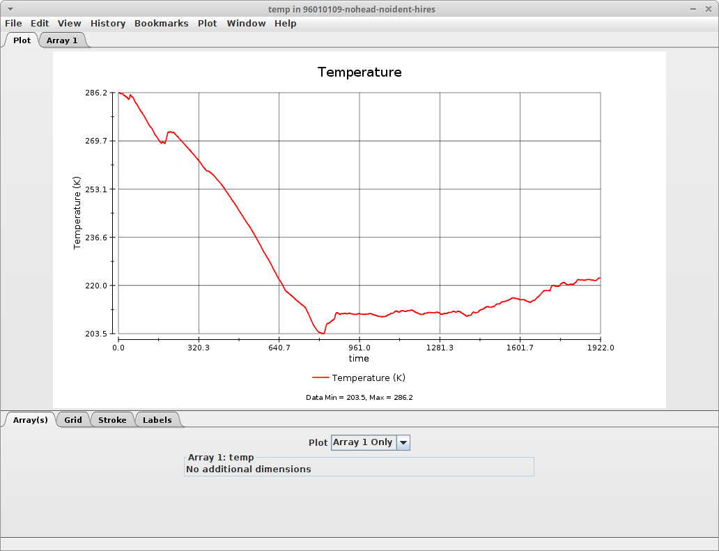
The following plot was created for the temperature found in one of these files, during the whole profiling of a radiosonde. You can see that as the radiosonde goes up in the atmosphere, the temperature decreases, but then increases again. Which is normal when you move beyond the tropopause.

That’s all for today!
Categories: Blog
Tags: Python